Many important problems are not naturally arranged as rows in a table or pixels in an image. They are made of entities and relationships.
A molecule is atoms connected by bonds. A traffic system is roads connected by intersections. A social network is people connected by relationships. A physical system is objects interacting through forces. A knowledge graph is facts connected through typed relations.
Graph Neural Networks, or GNNs, are neural networks designed for this kind of data.
Instead of assuming that every input is a fixed-size vector or grid, a GNN treats the input as a graph: nodes represent entities, edges represent relations, and optional global features describe the whole system.
Why Graphs Need Their Own Neural Networks
Standard neural networks usually assume a fixed structure.
A convolutional neural network assumes a grid, such as an image. A transformer assumes a sequence or set of tokens. A multilayer perceptron assumes a fixed-size vector.
Graphs are different. They can have:
- different numbers of nodes
- different numbers of edges
- different connectivity patterns
- directed or undirected relations
- node-level, edge-level, and graph-level attributes
This makes graphs flexible, but it also makes them harder to process with standard architectures.
GNNs solve this by learning through message passing. Nodes exchange information with their neighbors. Edges help define how information flows. After several rounds of message passing, each node has a representation that reflects both its own features and the surrounding graph structure.
Where GNNs Are Used
GNNs are useful whenever relationships matter.
Common applications include:
- molecular property prediction
- drug discovery
- traffic forecasting
- recommendation systems
- knowledge graph reasoning
- social network analysis
- scene understanding
- physical simulation
- multi-agent systems
- program analysis
- combinatorial optimization
- 3D meshes and point clouds
- semi-supervised node classification
They are also useful in neuro-symbolic AI because graphs can represent symbolic structure: entities, relations, facts, constraints, proof steps, or object interactions.
What Is a Graph?
In the graph network framework, a graph is represented as:
G = (u, V, E)
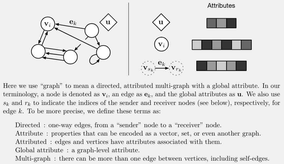
The three parts are:
u: global attributes for the whole graphV: a set of nodesE: a set of edges
A node v_i represents an entity. It may contain features such as object type, position, mass, label, or hidden state.
An edge e_k represents a relation from a sender node to a receiver node. It may contain features such as distance, bond type, interaction strength, or relation type.
The global attribute u stores information about the whole graph. In a physical simulation, this might be gravity or time step. In a molecular graph, it might be temperature or environment. In a scene graph, it might describe the overall scene.
This node-edge-global structure is powerful because many tasks require all three levels.
The Graph Network Block
The paper “Relational Inductive Biases, Deep Learning, and Graph Networks” by Battaglia et al. presents a general graph network block. The idea is simple: take a graph as input, update its edges, nodes, and global attributes, then output an updated graph.
This makes the block a graph-to-graph module.
Internal Structure
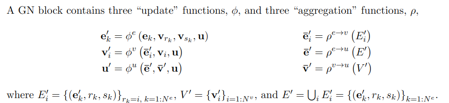
A graph network block has update functions and aggregation functions.
The update functions are:
phi_e: updates edge attributesphi_v: updates node attributesphi_u: updates global attributes
The aggregation functions are:
rho_e_to_v: aggregates incoming edge information for each noderho_e_to_u: aggregates edge information for the whole graphrho_v_to_u: aggregates node information for the whole graph
Aggregation functions must be permutation-invariant. That means the result should not depend on the arbitrary ordering of nodes or edges. Sum, mean, max, and attention-style pooling are common examples.
This matters because a graph is a set-like structure. Reordering the node list should not change the meaning of the graph.
Message Passing: The Core Idea
The easiest way to understand GNNs is to think in terms of messages.
Each edge computes a message from its sender node, receiver node, edge features, and global context. Each node receives messages from neighboring edges and aggregates them. The node then updates its own representation. Finally, the graph can update its global representation using information from all nodes and edges.
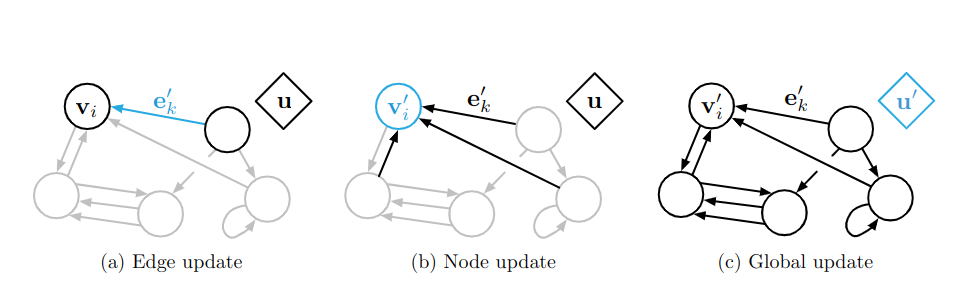
This process lets information move through the graph.
After one message-passing step, a node knows about its immediate neighbors. After two steps, it can receive information from neighbors of neighbors. After more steps, information can travel farther.
This is why GNN depth is related to graph distance. A shallow GNN captures local structure. A deeper GNN can capture broader graph context, though very deep GNNs can suffer from oversmoothing or optimization problems.
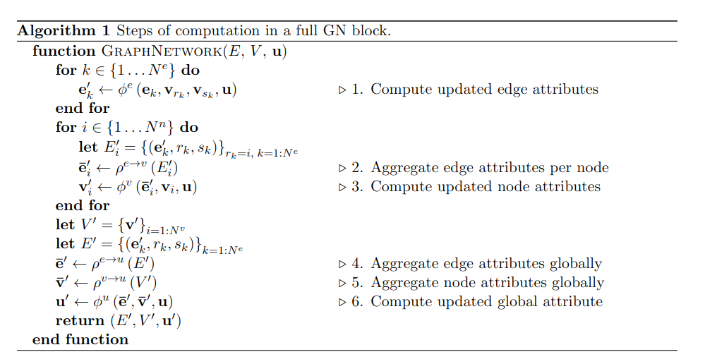
Computational Steps in a Graph Network Block
The graph network block usually updates information in this order:
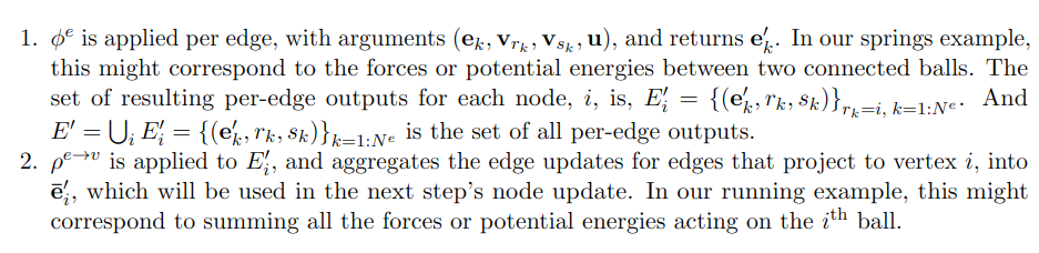
- Update edges.
- Aggregate edge information for each receiver node.
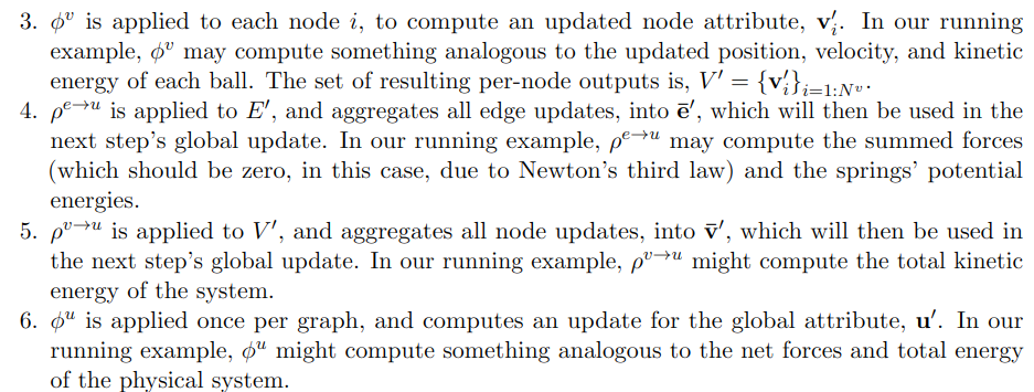
- Update nodes.
- Aggregate edge and node information for the global attribute.
- Update the global attribute.
The edge update can use:
- the old edge feature
- the sender node feature
- the receiver node feature
- the global feature
The node update can use:
- the old node feature
- the aggregated incoming edge messages
- the global feature
The global update can use:
- the old global feature
- aggregated edge information
- aggregated node information
This design is general. Different GNN models can be seen as special cases depending on which parts are used.
Algorithm View
The algorithm form makes the modularity clear. A graph network block applies learned functions to each edge, each node, and the graph-level state.
Because the same functions are reused across all edges and nodes, the model can process graphs of different sizes. This is one reason GNNs are attractive for combinatorial generalization.
For example, a model trained on small physical systems may generalize to larger systems if the learned local interaction rule is reusable. This idea is important in scientific machine learning and appears again in Learning Symbolic Physics with Graph Networks.
Relational Inductive Bias
An inductive bias is an assumption built into a model that helps it learn.
CNNs have a spatial inductive bias: nearby pixels matter, and the same filters can be reused across an image.
GNNs have a relational inductive bias: entities interact through relations, and the same interaction function can be reused across the graph.
This gives GNNs three important properties.
First, interaction is controlled by graph structure. If two nodes are connected, they can exchange messages. If they are not connected, they do not directly interact. The model’s computation follows the relational structure of the input.
Second, nodes and edges are treated as sets. The model does not depend on arbitrary ordering. This is essential for graphs because node order usually has no meaning.
Third, update functions are shared. The same edge update is applied to all edges, and the same node update is applied to all nodes. This supports generalization to new graph sizes and connectivity patterns.
These biases make GNNs especially useful for systems where the same kind of local relation repeats many times: atoms in molecules, vehicles in traffic, objects in scenes, agents in a swarm, or bodies in a physical simulation.
Node, Edge, and Graph-Level Tasks
GNNs can be used for different prediction targets.
In node-level tasks, the goal is to predict something about each node. Examples include classifying users in a social network, labeling papers in a citation graph, or identifying objects in a scene.
In edge-level tasks, the goal is to predict something about relationships. Examples include link prediction, relation classification, and interaction prediction.
In graph-level tasks, the goal is to predict something about the whole graph. Examples include molecular property prediction, graph classification, program behavior prediction, or physical system forecasting.
The graph network framework supports all three because it maintains node, edge, and global representations.
Common Challenges
GNNs are powerful, but they are not automatic solutions.
One challenge is graph construction. The model only reasons over the graph it receives. If important edges are missing or wrong, the GNN may learn the wrong interactions.
Another challenge is oversmoothing. After many message-passing layers, node representations can become too similar, making it hard to distinguish nodes.
There is also oversquashing, where too much distant information is compressed through narrow graph bottlenecks.
Scalability is another issue. Very large graphs require sampling, batching, or approximate methods.
Finally, explanations can be difficult. A GNN follows graph structure, but its learned messages may still be opaque. For high-stakes applications, we need tools to inspect which nodes, edges, and subgraphs influenced a prediction.
Why GNNs Matter for Neurosymbolic AI
Graphs are one of the most natural bridges between neural learning and symbolic structure.
Symbolic AI often represents knowledge as objects and relations. GNNs can process objects and relations with neural learning. This makes them useful for knowledge graphs, scene graphs, program graphs, proof graphs, molecular graphs, and physical interaction graphs.
In neuro-symbolic systems, a GNN can serve as the learned relational engine. It can process structured symbolic input while still benefiting from gradient-based learning.
That is why GNNs appear repeatedly in modern work on symbolic reasoning, scientific discovery, relational learning, and interpretable AI.
Takeaway
Graph Neural Networks are neural models for relational data.
They represent systems as nodes, edges, and global attributes. They learn by passing messages along graph connections. Their main strength is relational inductive bias: the model assumes that entities and relationships matter, and it structures computation accordingly.
This makes GNNs useful wherever the problem is naturally about interactions: molecules, scenes, traffic, physics, programs, knowledge graphs, social networks, and multi-agent systems.
The central idea is simple:
When the world is relational, the model should be relational too.
References
- Battaglia, P. W., Hamrick, J. B., Bapst, V., Sanchez-Gonzalez, A., Zambaldi, V., Malinowski, M., Tacchetti, A., Raposo, D., Santoro, A., Faulkner, R., Gulcehre, C., Song, F., Ballard, A., Gilmer, J., Dahl, G., Vaswani, A., Allen, K., Nash, C., Langston, V., Dyer, C., Heess, N., Wierstra, D., Kohli, P., Botvinick, M., Vinyals, O., Li, Y., and Pascanu, R. (2018). Relational inductive biases, deep learning, and graph networks. arXiv:1806.01261.