Decision trees are popular because they are easy to understand: start at the root, ask a question, move left or right, and keep going until a leaf gives the final prediction. That simplicity is also their weakness. A hard split creates a sharp boundary. Two points that are almost identical can fall on different sides of a threshold and receive very different predictions.
The paper “Soft Decision Trees” by Ozan Irsoy, Olcay Taner Yildiz, and Ethem Alpaydin, published at ICPR 2012, proposes a smoother version of this idea. Instead of sending an input down exactly one branch, a soft decision tree sends it down both branches with different probabilities. Every leaf can contribute to the output, but some leaves matter much more than others.
That small change makes the tree behave less like a set of abrupt rules and more like a weighted mixture of local predictions.
The Problem with Hard Decisions
In a standard binary decision tree, each internal node applies a test to the input. If the test is true, the input goes to the left child. Otherwise, it goes to the right child.
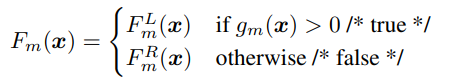
This gives the model a very clear structure. For classification, the leaf usually stores a class label or class distribution. For regression, the leaf stores a numeric value. The prediction is made by one path from the root to one leaf.
That path-based behavior is useful when the true decision boundary is naturally rule-like. But for many real datasets, the target function changes gradually. In regression especially, hard trees often need many small leaves to approximate a smooth curve. The model remains interpretable at each split, but the full tree can become large and fragmented.
The Soft Tree Idea
A soft decision tree keeps the tree structure but changes what happens at an internal node. Instead of choosing only one child, the node computes a probability for the left child and a probability for the right child. The output of the node is then a weighted combination of the outputs of both subtrees.

In the binary case, the gating function produces a value between 0 and 1:
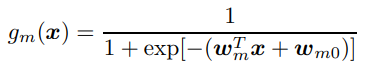
Here, the gating function is a sigmoid applied to a linear function of the input. If the gate returns a value close to 1, the left subtree dominates. If it returns a value close to 0, the right subtree dominates. If it returns something near 0.5, both sides matter.
So the tree is still making decisions, but the decisions are no longer all-or-nothing.
How the Prediction Is Computed
The response of a soft tree is computed recursively. A leaf returns its stored value. An internal node calls both children, weights their outputs by the gate, and returns the weighted sum.
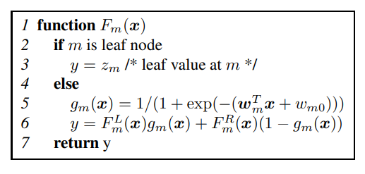
This means every root-to-leaf path is considered. A leaf’s contribution is controlled by the product of the gating probabilities along the path that reaches it.
For example, if a leaf is reached through three soft gates, and those gates assign probabilities of 0.8, 0.6, and 0.9 to that path, the leaf contributes with weight 0.8 * 0.6 * 0.9. Other leaves contribute too, but with their own path weights.
This is the key difference from a hard tree. A hard tree asks, “Which leaf owns this example?” A soft tree asks, “How much should each leaf contribute?”
Training the Tree
The paper trains the tree incrementally, much like a normal decision tree. It starts with a single leaf that predicts a constant value. Then it tries to replace a leaf with a small subtree: one internal soft decision node and two new leaf nodes.
The model uses different loss functions depending on the task:
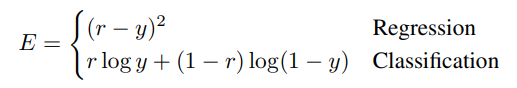
For regression, the objective is squared error. For classification, the objective is cross-entropy. The paper focuses on two-class classification, where the final tree output can be interpreted as a probability.
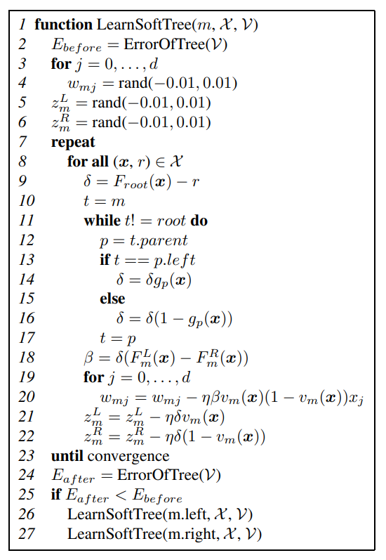
The training step optimizes three things for a candidate split:
- the gate parameters at the internal node
- the value stored in the left child
- the value stored in the right child
These parameters are learned with gradient descent. A validation set decides whether the proposed split should actually be kept. If the split improves validation performance, the algorithm accepts it and recursively tries to grow the two children. If it does not improve validation performance, the node stays as a leaf.
This gives the method a useful safeguard: the tree grows only when a new soft split earns its place.
Why Initialization Matters
The authors found that starting gradient descent from random values worked poorly. That is not surprising. A soft tree has a non-convex training objective, so bad initialization can send optimization into weak local minima.
Their practical solution is clever: first find the split that a hard decision tree would have used, then initialize the soft gate from that split. The initial gate is therefore a softened version of a reasonable hard rule. Gradient descent then refines it.
This makes the method more stable. The model begins with a decision boundary that already separates the data somewhat well, then learns how sharp, tilted, or smooth that boundary should be.
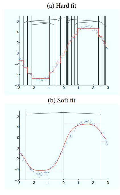
What the Toy Example Shows
The paper visualizes the difference on a noisy sinusoidal regression dataset.
The hard decision tree needs 37 nodes and 19 leaves to fit the curve. The soft decision tree reaches comparable accuracy with only 7 nodes and 4 leaves.
That difference is important. The soft tree does not need to create many tiny constant regions, because the sigmoid gates interpolate smoothly between neighboring leaves. A smaller tree can represent a smoother function.
In other words, soft routing reduces the need for extra leaves whose only job is to patch the discontinuities created by hard splits.
Regression Results
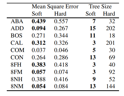
The regression experiments are the strongest part of the paper. Across ten regression datasets, the soft tree uses significantly fewer nodes than the hard tree on every dataset. In most cases, it also achieves lower mean squared error.
This matches the intuition behind the method. Regression problems often involve smooth target functions, and hard trees struggle with smoothness because each leaf predicts a constant value. Soft trees still use constant leaves, but the gates blend those leaves together, producing a smoother response.
There is a cost: a prediction in a soft tree visits all paths rather than one path. But because the resulting tree can be much smaller, the extra computation at each node may be offset by the reduction in tree size.
Classification Results
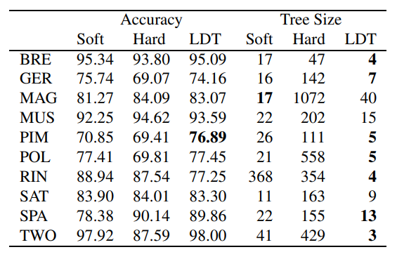
The classification results are more mixed. The soft tree wins on three datasets, the hard tree wins on two, and the remaining five are ties. So the paper does not show a universal classification advantage in accuracy.
However, model size still improves. Soft trees are generally smaller than hard trees, although linear discriminant trees are often smaller still. The comparison is not perfectly apples-to-apples because the pruning strategies differ, but the overall message is clear: soft decisions can reduce tree complexity without necessarily sacrificing accuracy.
For classification, the benefit depends on the shape of the boundary. If the class boundary is naturally sharp, a hard split can work well. If the boundary is gradual or noisy, soft routing may give a more robust model.
Why Soft Trees Are Useful
Soft decision trees sit in an interesting middle ground.
They preserve some of the structure of decision trees: internal nodes, leaves, recursive prediction, and a visible hierarchy. At the same time, they borrow ideas from neural networks: differentiable gates, weighted combinations, and gradient-based optimization.
The main advantages are:
- smoother predictions near split boundaries
- fewer nodes for many regression problems
- oblique splits through linear gating functions
- a natural connection to mixture-of-experts models
- differentiability, which allows gradient-based learning
The oblique split point is worth emphasizing. A standard univariate tree usually splits on one feature at a time. A soft decision node uses a linear function of all features before applying the sigmoid, so the split can be angled in feature space. This can reduce the number of nodes needed to express a decision boundary.
Limitations
Soft trees also give up some of the simplicity of classic trees.
A hard tree is easy to trace: one input, one path, one leaf. A soft tree uses all paths, which makes a single prediction harder to explain locally. You can still inspect the gates and leaf contributions, but the explanation is now a weighted mixture rather than a crisp rule chain.
Training is also more delicate. Gradient descent can get stuck in local minima, and performance depends on initialization and learning-rate choices. The paper’s hard-split initialization helps, but it does not remove the optimization challenge entirely.
Finally, a soft tree can be more expensive at prediction time if the tree is large, because all leaves may contribute. The method is most attractive when soft routing allows the tree to remain compact.
Connection to Distillation
This 2012 paper is about learning soft decision trees directly from data. A related line of work uses soft decision trees as interpretable students trained to mimic neural networks.
I covered that idea separately in Distilling a Neural Network Into a Soft Decision Tree. The two ideas are closely related, but the motivation is different. Here, the goal is a smoother and smaller tree model. In distillation, the goal is often to approximate a trained neural network with a more interpretable tree-like model.
Takeaway
The central idea of soft decision trees is simple: do not force every internal node to make a hard choice. Let both branches contribute, and learn how strongly each branch should matter.
That change makes the model smoother, more flexible, and often smaller. The paper’s results suggest that the approach is especially useful for regression, where gradual interpolation between leaves can capture structure that hard trees approximate only by growing many extra nodes.
Soft decision trees are not a full replacement for classic decision trees. They are less crisp, harder to optimize, and slightly harder to explain path-by-path. But they are a useful bridge between symbolic tree structure and differentiable learning, which is exactly why they remain interesting in modern interpretable machine learning and neuro-symbolic AI.
References
- Irsoy, O., Yildiz, O. T., and Alpaydin, E. (2012). Soft Decision Trees. Proceedings of the 21st International Conference on Pattern Recognition (ICPR 2012), 1819-1822. IEEE.