The gravity model is one of the classic tools in transportation planning. It helps answer a simple but important question: once we know how many trips are produced in each zone and how many trips are attracted to each zone, how should those trips be distributed between origins and destinations?
In other words, the gravity model helps turn trip ends into trip flows.
The idea is borrowed from Newton’s law of gravity. Bigger places tend to interact more, and places that are farther apart tend to interact less. In transportation, “bigger” usually means more people, jobs, services, shopping, schools, or other trip-attracting activity. “Farther apart” usually means higher travel time, distance, cost, or inconvenience.
Where the Gravity Model Fits
In the traditional four-step travel demand model, gravity models are used in the trip distribution step.
The four steps are:
- Trip generation: estimate how many trips each zone produces and attracts.
- Trip distribution: connect those productions and attractions into zone-to-zone flows.
- Mode choice: estimate whether travelers use car, transit, walking, biking, air mobility, or other modes.
- Assignment: load those trips onto specific routes or networks.
The gravity model operates mainly in step two. It takes trip productions and trip attractions and estimates a trip table, often called a production-attraction table or OD-style matrix after later processing.
The Basic Gravity Model
The basic form says that interaction between two zones increases with the size of the origin and destination and decreases with travel impedance.
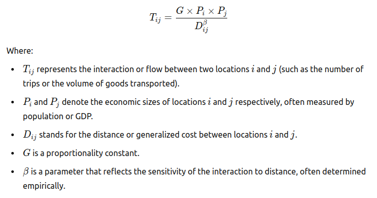
In transportation terms, the model says:
- A zone with more trip productions sends out more trips.
- A zone with more trip attractions receives more trips.
- Trips are less likely when travel time, distance, or cost increases.
This is why two large nearby areas usually have more interaction than two small distant areas.
Productions and Attractions
Productions and attractions are not always the same as origins and destinations.
For home-based trips, the home end is often treated as the production end, even if the person is returning home in the evening. The workplace, school, shop, or service location is treated as the attraction end.
This convention is useful for modeling daily travel patterns. A residential zone with many households produces many trips. An employment center with many jobs attracts many trips. The gravity model then distributes those trips based on both attraction strength and travel impedance.
Impedance and Friction Factors
The impedance term is the heart of the gravity model. It represents the difficulty of traveling between two zones.
Impedance can be measured as:
- Distance.
- Travel time.
- Generalized cost.
- Transit travel time.
- Auto travel time.
- A combined measure of time, cost, transfers, parking, and reliability.
In practice, travel time is often used because it strongly affects destination choice. A friction factor is then applied to represent how willingness to travel declines as impedance increases.
Short trips usually have high friction-factor values because they are easy to make. Long trips usually have low friction-factor values because fewer people are willing to make them.
Extending the Gravity Model
The extended gravity model introduces calibration parameters to better fit observed travel behavior.
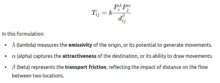
The article’s earlier draft described these parameters as lambda, alpha, and beta. A practical way to interpret them is:
lambda: the trip-producing strength of an origin.alpha: the attractiveness of a destination.beta: the sensitivity to travel impedance.
For example, a dense residential district may have high production strength because many people live there. A downtown employment center may have high attractiveness because many jobs are located there. A corridor with poor travel conditions may have high friction because travel between zones is slow or inconvenient.
These parameters are not universal constants. They must be calibrated for the region, trip purpose, time period, and mode being modeled.
Calibration
Calibration is what makes a gravity model useful rather than just intuitive.
Planners compare the model’s predicted trip length distribution with observed travel data. If the model predicts too many long trips, the friction factors may need to be adjusted. If it predicts too many short trips, the impedance sensitivity may be too strong.
Gravity models are often calibrated separately by trip purpose. Work trips, shopping trips, school trips, and recreational trips do not have the same distance tolerance. A person may travel much farther for a job than for a grocery store.
The model may also need balancing so that predicted trips leaving each production zone and arriving at each attraction zone match the trip generation totals.
Why Congested Travel Times Matter
A common issue is whether to use free-flow travel time or congested travel time.
If the model uses free-flow times, it may overestimate the attractiveness of trips that are actually slow during peak periods. If it uses congested times, it better reflects real travel friction. For that reason, planning guidance often encourages iterating between trip distribution and assignment until travel times stabilize.
This feedback matters because the gravity model can shift demand based on impedance, and the assigned demand can change impedance by creating congestion.
Applications
Gravity models are used in many transportation and spatial-analysis tasks.
In urban planning, they help estimate how new housing, jobs, schools, hospitals, or shopping centers may change regional travel patterns.
In highway and transit planning, they help produce trip tables that can be assigned to networks for congestion, capacity, and investment analysis.
In freight planning, gravity-style models can estimate goods movement between production and consumption areas.
In regional air mobility or advanced air mobility studies, gravity models can help estimate potential flows between cities, airports, vertiports, or activity centers when direct demand data is unavailable.
Why the Model Remains Popular
Gravity models remain popular because they are simple, interpretable, and relatively data-efficient.
They require three main ingredients:
- Trip productions by zone.
- Trip attractions by zone.
- Travel impedance between zones.
That makes them practical for regions where detailed behavioral data is limited. They also provide a transparent baseline for understanding how size and separation shape travel demand.
Limitations
The same simplicity that makes the gravity model useful also limits it.
The model may miss important behavioral factors such as income, car ownership, parking cost, transit quality, land-use mix, walkability, safety, household structure, destination variety, and traveler preferences.
It can also struggle with barriers that are not well represented by distance or travel time. A river, mountain, toll, poor transit connection, or social boundary may reduce interaction more than the basic impedance term suggests.
Gravity models may also produce unrealistic responses when transportation service changes. More advanced destination choice models often perform better because they can include richer explanatory variables and a stronger behavioral foundation.
Gravity Models vs. Destination Choice Models
Destination choice models are often viewed as a more flexible modern alternative. They use discrete choice methods to estimate the probability that a traveler chooses a destination based on travel time, cost, attractiveness, accessibility, and traveler characteristics.
Gravity models can be interpreted as a simpler special case of spatial interaction modeling. They are still useful, especially for sketch planning or regions with limited data, but many larger metropolitan models have moved toward destination choice methods for improved behavioral realism.
That does not make gravity models obsolete. It means planners should understand what the model can and cannot explain.
Final Thoughts
The gravity model is powerful because it captures a basic truth of travel: people and goods move more between places that are attractive and accessible.
Its strength is clarity. Productions, attractions, and impedance provide a simple framework for estimating spatial interaction. Its weakness is that real travel behavior is more complex than size and distance alone.
For transportation planning, the gravity model is best used as a structured, calibrated approximation. It can help build trip tables, test scenarios, and understand regional connectivity, but its assumptions should always be checked against observed data and local context.
References
- Travel Forecasting Resource, Trip Distribution. https://tfresource.org/topics/Trip_distribution
- Federal Highway Administration, Model Destination Choice. https://www.fhwa.dot.gov/planning/tmip/publications/other_reports/model_destination_choice/index.cfm
- Transportation Research Board, NCHRP Report 365: Travel Estimation Techniques for Urban Planning. https://onlinepubs.trb.org/onlinepubs/nchrp/nchrp_rpt_365.pdf